Nonnegative Matrix Factorization, 1
The aim of this post is to highlight the utility of non-negative factorization (NMF) in data analysis through examples. In a different post, we’ll talk theory and implementation by thinking of NMF as constrained optimization.
Learning parts of a whole
When Lee and Seung [Lee99] re-introduced non-negative matrix factorization (NMF), they emphasized on the algorithm’s ability to learn parts of a whole. That is, a good and interpretable low-rank approximation of a function or data e.g. features of a face or the semantic components of text. Moreover, in interpreting the algorithm as a neural network, they argue that the part-based learning is a consequence of the non-negativity constraint (neuron firing rates and synaptic strengths are non-negative). This is contrasted with well-known techniques such as Principle Component Analysis (PCA) and Vector Quantization (VQ), which learn by creating archetypes of objects. In all three cases, the algorithms model data as a linear and additive combination of “basis” functions or vectors - the difference lying in the constraints imposed on the model.
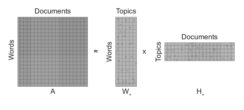
Thus, given an $n \times m$ data matrix $V$, we seek matrix factors $W$ and $H$, which are $n \times k$ and $k \times m$, respectively such that some loss function (one below is for Frobenius norm) is minimized for a given value of $k$:
In some ways, the issues raised by Lee99 were not new. In chemometrics and environmetrics, NMF was already being used for analyzing molecular spectra Juvela94 and receptor modeling [Hopke00]. This was motivated by the (1) lack of interpretation for factors produced by PCA (which, when addressed by matrix rotations can cause the problem to have non-unique solutions), and (2) the sensitivity of PCA to data scaling. The latter issue is connected with the need to account for uncertainty in data, which is harder to achieve with PCA yet important for modeling in those areas:
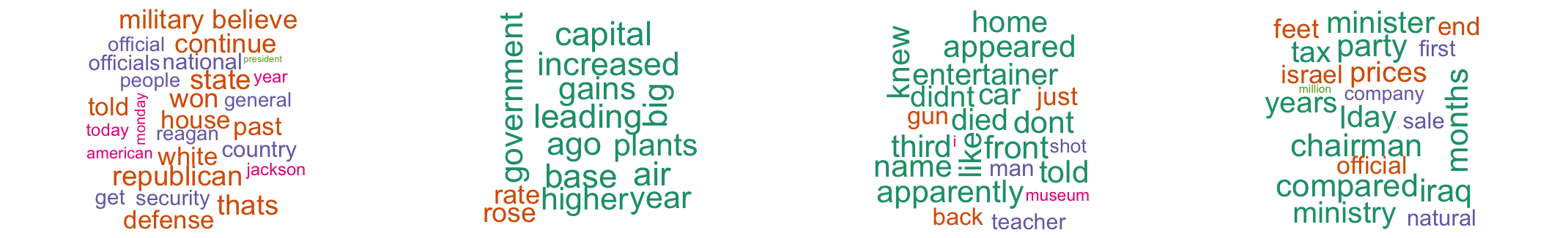
Here’s R code for latent semantic indexing using the excellent NMF package. The dataset used is AssociatedPress (from topicmodel package), which is available as a DocumentTermMatrix (see the TM package) encoding the TF-IDF of terms in various documents. NMF is calculated for a vector of four factors and then the terms closet to each factor are drawn as a word cloud (see the wordcloud package).
library(topicmodels)
library(tm)
library(NMF)
library(wordcloud)

data(AssociatedPress)
dtm <- AssociatedPress[1:20,]
dtm <- removeSparseTerms(dtm, 0.9)
dm <- as.matrix(dtm)
dim(dm)

k <- 4
nmf.res <- nmf(dm, k, "snmf/r")
basismap(nmf.res)
coefmap(nmf.res)

# top basis and coefficients
res.coef <- coef(nmf.res)
res.bas <- basis(nmf.res)

set.seed(1234)
for (n in seq(1, k, 1)) {
 freq <- res.coef[n,(order(res.coef[n,], decreasing = TRUE) [1:40])]
 wordcloud(names(freq), round(freq), scale = c(0.1, 3), colors = brewer.pal(6, "Dark2"))
 print(freq)
 print("==========================")
}
Summary: NMF is useful because some applications (e.g. in physical sciences and signal processing) naturally restrict the data and hence latent factor to be non-negative, and NMF can satisfy this constraint.
Collaborative filtering
While NMF steadily found new applications in diverse fields such as signal processing and data mining [Cichoki09], perhaps matrix factorization’s role in solving the Netflix prize problem [Koren09, or this summary made it more prominent within machine learning communities. Koren09 starts out with distinguishing two types of learning models for collaborative filtering: neighborhood and latent factor. Neighborhood models find similarity between users or between items, whereas latent factor models find variables that can explain both user preferences and item characteristics. Within latent factor models, the authors focus on SVD (instead of NMF, perhaps because, unlike physical science, negative ratings are not much of a concern here). Classical SVD’s disadvantage seems to lies in not being able to handle missing entries in the data (user-item matrix). Drawing on previous work, they argue for the need to (1) fit model based on known data value alone, and (2) avoid overfitting using regularization.
The basic model, then, according to Koren09 is the following optimization problem:
where $v_{ij}$ is the rating for item $j$ by user $i$, $w_i$ is the user’s factor vector, $h_j$ the item’s factor vector, and $\lambda$ is the regularization parameter.
The paper also highlights two interesting extensions to the basic model:
- Biases: $ \hat{v_{ij}} = \mu + b_i + b_j + w_{i}^{T} h_{j} $
- Temporal dynamics: $ \hat{v_{ij}}(t) = \mu + b_{i}(t) + b_{j}(t) + w_{i}^{T} h_{j} $
The Netflix prize is also a Matrix Completion problem that we can solve using NMF (though factorizing first might be more inefficient). Here’s R code for collaborative filtering based on the MovieLens 100K dataset (“100,000 ratings from 1000 users on 1700 movies”). Much of the code is involved with reading and parsing the MovieLens data and metadata, and draws on ggplot2 and directlabels for visualization.
# read the Movie Lens data from file
u1.base <- read.table(file="~/Desktop/mlearn/Rcode/ml-100k/u1.base",sep='\t',header=F, col.names=c("userId", "itemId", "rating", "timestamp"), colClasses = c("integer", "integer", "integer", "integer"))
# get all unique users and items
unq.users <- sort(unique(u1.base$userId))
unq.items <- sort(unique(u1.base$itemId))
library(bit64)
unq.users.i64 <- as.integer64(unq.users)
unq.items.i64 <- as.integer64(unq.items)
# hashmaps store the index of each user and item
users.hm <-hashmap.integer64(unq.users.i64, nunique = length(unq.users.i64))
items.hm <-hashmap.integer64(unq.items.i64, nunique = length(unq.items.i64))
# populate the ratings matrix
u1.base.mat <- matrix(data = 0, nrow = length(unq.users.i64), ncol = length(unq.items.i64))
for (i in 1:nrow(u1.base)) {
u1.base.mat[hashpos(users.hm, u1.base[i,1]), hashpos(items.hm, u1.base[i,2])] <- u1.base[i,3]
}
rownames(u1.base.mat) <- unq.users
colnames(u1.base.mat) <- unq.items
# factorize, with as many factors as movie genres given in the ML data
library(NMF)
k <- 19
set.seed(8888)
nmf.res <- nmf(u1.base.mat, nrun = 5, rank = k, method = "snmf/r")
basismap(nmf.res)
coefmap(nmf.res)
# top basis and coefficients, and metadata
res.coef <- coef(nmf.res)
res.bas <- basis(nmf.res)
item.col.names = c("movieId", "movieTitle", "releaseDate", "vidReleaseDate", "imdbUrl",
"unknown", "Action", "Adventure", "Animation",
"Children", "Comedy", "Crime", "Documentary", "Drama", "Fantasy",
"FilmNoir", "Horror", "Musical", "Mystery", "Romance", "SciFi",
"Thriller", "War", "Western")
item.col.classes = c("integer", "character", "character", "character", "character",
"integer", "integer", "integer", "integer", "integer", "integer", "integer",
"integer", "integer", "integer", "integer", "integer", "integer", "integer",
"integer", "integer", "integer", "integer", "integer")
# read.table does not work without "latin1" encoding and disabling quotes
u.item.txt <- readLines("~/Desktop/mlearn/Rcode/ml-100k/u.item", encoding = "latin1")
u.items <- read.table(text=u.item.txt,sep='|',header=F, col.names=item.col.names, colClasses = item.col.classes, encoding = "latin1", quote = "")
u.items[1,]
u.items[order(res.coef[1,], decreasing = TRUE) [1:20], 2]
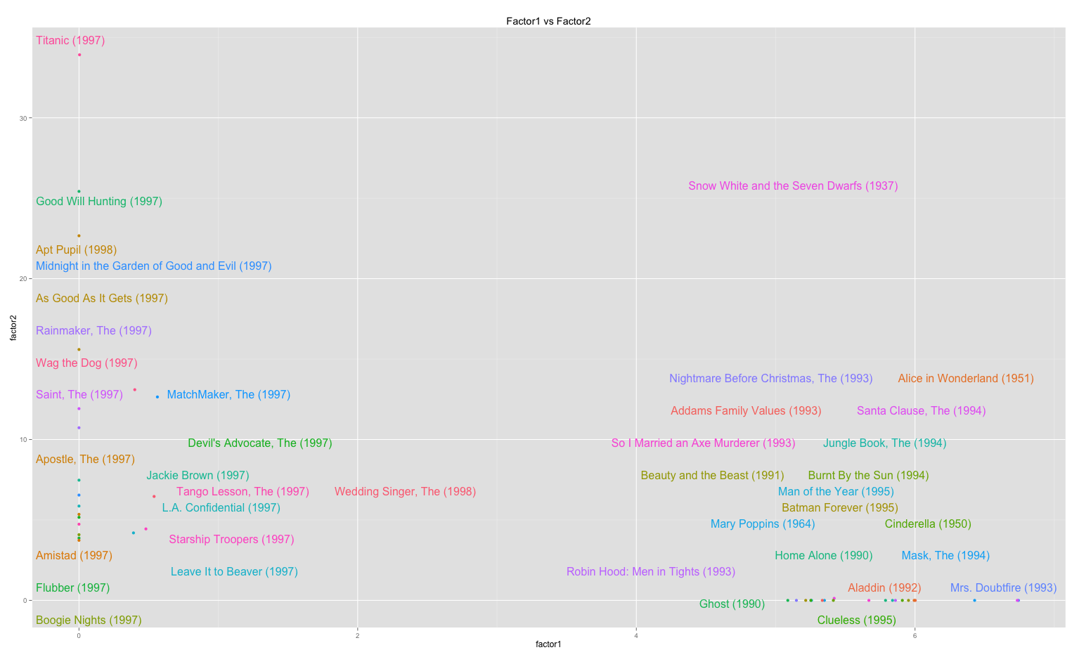
# scatterplot: one factor against another (as in Koren09)
factor1.idx <- order(res.coef[1,], decreasing = TRUE) [1:20]
factor2.idx <- order(res.coef[2,], decreasing = TRUE) [1:20]
plot.idx <- union(factor1.idx, factor2.idx)
qplot.dat <- data.frame(factor1 = res.coef[1, plot.idx], factor2 = res.coef[2, plot.idx], labels = u.items[plot.idx,2])
library(ggplot2)
library(directlabels)
plot.obj <-qplot(factor1, factor2, data=qplot.dat, colour = labels, main="Factor1 vs Factor2")
direct.label(plot.obj)
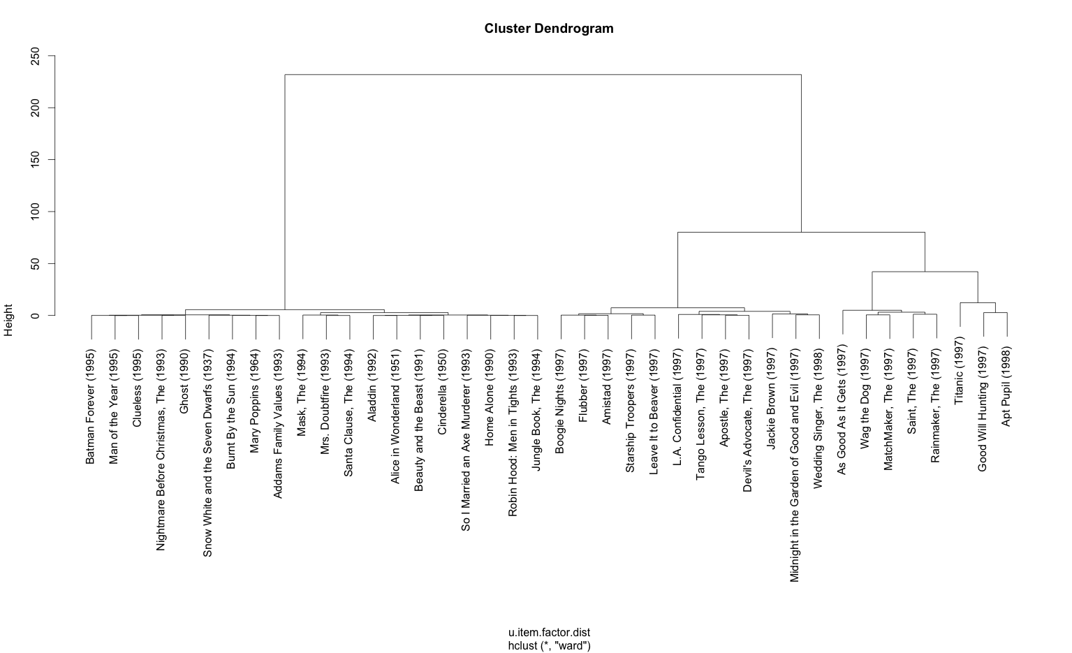
# plot hierarchical clusters for two factors
u.item.factor <- t(res.coef)
rownames(u.item.factor) <- as.list(u.items[1:nrow(u.item.factor),2])
u.item.factor.sampled <- u.item.factor[plot.idx,1:2]
u.item.factor.dist = dist(u.item.factor.sampled, method = "manhattan")
u.item.factor.clust = hclust(u.item.factor.dist, method = "ward")
plot(u.item.factor.clust)
The scatterplot and dendogram outputs of the code:
 |  |
Caveat: while NMF itself can be used for matrix completion, the NMF package in R cannot since it cannot account for missing values. An alternative is to use softImpute.
Summary: another reason for the success of NMF is the ability to extend the basic model for use in specific applications (like collaborative filtering).
Cluster analysis
Non-negative matrix factorization is essentially a form of cluster analysis - the critical difference being that the clusters are derived from linear, additive latent factors instead of item-to-item similarity/distance metrics/divergences. So, it’s not surprising that researchers were interested in the connections between traditional unsupervised learning methods like K-means and NMF. Two interesting papers in this line are Kim07 and Kim08. Apart from analyzing the relationship between K-mean and NMF, they highlight (though, not introduce):
- the importance of sparsity,
- utility of purity and entropy metrics to evaluate clustering quality, and
- the utility of of consensus maps Burnet04 for model selection
NMF, contrary to Lee and Seung’s intuition and experiments, doesn’t always produce a part-based representation. In this, Kim07 and Kim08 followed the arguments and counter-examples of Li01 and Hoyer04. Since, as Hoyer04 states, “the sparseness given by NMF is somewhat of a side-effect rather than a goal,” regularization needs to be explicitly introduced to control the degree of sparseness. Li07 does that by penalizing the energy of the factors in the optimization objective (similar to the Koren09 basic model); Hoyer04 introduces sparseness constraints separately on each factor; while Kim07, Kim08 mix $L_1$ and $L_2$ norms to impose sparsity on one of the factors. Sparseness may not only improve the quality of the result but, as Kim08 show, also result in better execution time. The two algorithms, SNMF/R and SNMF/L, introduced in Kim07 are available in the R NMF package.
Purity and entropy are two traditional clustering metrics. Purity measures the accuracy of assignment ($n$ data point, $k$ clusters and $l$ classes) - larger value implies better clustering. Entropy measures the amount of information-theoretic order - smaller value is better.
For model selection (i.e. the number of factors to use), Burnet04 introduced consensus matrix and the related dispersion coefficient. Since NMF may not converge to the same solution on each run, consensus matrix (C) encodes the probability of assignment agreement over multiple runs. The dispersion coefficient is calculated as the “Pearson correlation of two distance matrices: the first, I-C , is the distance between samples induced by the consensus matrix, and the second is the distance between samples induced by the linkage used in the reordering of C.” Kim07 described a more comprehensible version of dispersion coefficient that only uses the consensus matrix. It’s value also lies between 0 and 1, and the higher the better (1 indicates complete consensus). The NMF package implements this version.
Here’s R code to analyze the iris dataset using the NMF package:
data(iris)
library(NMF)
ir <- t(as.matrix(iris[, 1:4]));

ir.res.k2 <- nmf(ir, 2, nrun =10, seed=12345, method = "lee")
ir.res.k3 <- nmf(ir, 3, nrun =10, seed=12345, method = "lee")
ir.res.k4 <- nmf(ir, 4, nrun =10, seed=12345, method = "lee")

p.k2 <- purity(ir.res.k2, iris[,5])
p.k3 <- purity(ir.res.k3, iris[,5])
p.k4 <- purity(ir.res.k4, iris[,5])
plot(2:4, c(p.k2, p.k3, p.k4), xlab = "factors", ylab = "purity")

e.k2 <- entropy(ir.res.k2, iris[,5])
e.k3 <- entropy(ir.res.k3, iris[,5])
e.k4 <- entropy(ir.res.k4, iris[,5])
plot(2:4, c(e.k2, e.k3, e.k4), xlab = "factors", ylab = "entropy")

par(mfrow=c(2,2))
consensusmap(ir.res.k2)
consensusmap(ir.res.k3)
consensusmap(ir.res.k4)

d.k2 <- dispersion(ir.res.k2)
d.k3 <- dispersion(ir.res.k3)
d.k4 <- dispersion(ir.res.k4)
plot(2:4, c(d.k2, d.k3, d.k4), xlab = "factors", ylab = "dispersion")

ir.res.k2.s <- nmf(ir, 2, nrun =10, seed=12345, method = "snmf/r")
ir.res.k3.s <- nmf(ir, 3, nrun =10, seed=12345, method = "snmf/r")
ir.res.k4.s <- nmf(ir, 4, nrun =10, seed=12345, method = "snmf/r")

d.k2.s <- dispersion(ir.res.k2.s)
d.k3.s <- dispersion(ir.res.k3.s)
d.k4.s <- dispersion(ir.res.k4.s)
plot(2:4, c(d.k2.s, d.k3.s, d.k4.s), xlab = "factors", ylab = "dispersion (snmf/r)")
This code uses the package’s heatmap tools: basismap, coefmap and consensusmap. If samples are taken to be the rows of a $n_m$ data matrix $V$ and features are taken to be its columns, then basismap draws the $n_k$ matrix factor W, which represents the contribution of each factor in each sample. Similarly, coefmap helps visualize the $k_m$ matrix factor $H$, which represents the contribution of each feature in each factor. Here are the rank-2 and rank-3 maps:
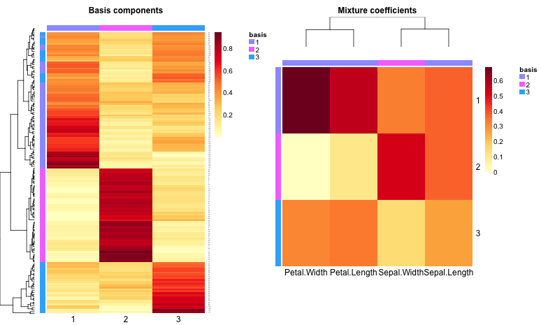 | 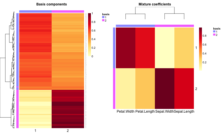 |
|---|---|
| Basis and coefficient maps for k = 3 | Basis and coefficient maps for k = 2 |
Not surprisingly, purity is maximized at $k = 3$ while entropy is minimized. Surprisingly, though, dispersion decreases as factors increase (also obvious from the consensusmap plots). Though Kim07, Kim08 don’t seem to discuss this, it may be that dispersion on its own is not reliable for model selection.
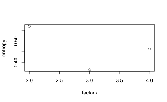 | 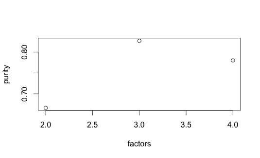 |
|---|---|
| k = 2-4, Entropy | k = 2-4, Purity |
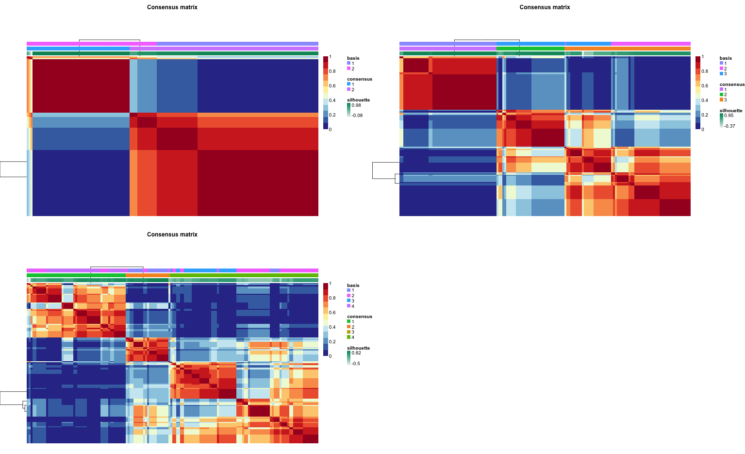 |
|---|
| Consensus matrics, k=2-4 |
Summary: NMF lends well to cluster analysis though model selection seems tricky.
References
- Arora12a S. Arora, R. Ge, R. Kannan, and A. Moitra. Computing a Nonnegative Matrix Factorization – Provably. STOC, 2012
- Arora12b S. Arora, R. Ge, A. Moitra. Learning Topic Models - Going Beyond SVD. FOCS, 2012
- Brunet04 J. Brunet, P. Tamayo, T. Golub, and J. Mesirov. Metagenes and molecular pattern discovery using matrix factorization. PNAS, 2004.
- Cichoki09 A. Cichoki, R. Zdunek, A. H. Phan, S. Ammari. Nonnegative Matrix and Tensor Factorizations: Applications to exploratory multi-way data analysis and blind source separation, 2009.
- Donoho03 D. Donoho and V. Stodden. When Does Non-Negative Matrix Factorization Give a Correct Decomposition into Parts? NIPS, 2003.
- Hopke00 P. K. Hopke. A guide to positive matrix factorization.Workshop on UNMIX and PMF as Applied to PM2, 2000.
- Hoyer04 P. O. Hoyer. Non-negative matrix factorization with sparseness constraints. JMLR, 2004.
- Juvela94 M. Juvela, K. Lehtinen, and P. Paatero. The use of positive matrix factorization in the analysis of molecular line spectra from the thumbprint nebula.
- [Clemens94] D. P. Clemens and R. Barvainis, eds., Clouds, Cores, and Low Mass Stars, volume 65 of ASP Conference Series, 1994.
- Juvela96 M. Juvela, K. Lehtinen, and P. Paatero. The use of positive matrix factorization in the analysis of molecular line spectra. MNRAS, 1996.
- Kim07 H. Kim and H. Park. Sparse non-negative matrix factorizations via alternating non-negativity-constrained least squares for microarray data analysis. Bioinformatics, 2007.
- Kim08 J. Kim and H. Park. Sparse Nonnegative Matrix Factorization for Clustering. Georgia Tech Technical Report, GT-CSE-08-01, 2008.
- Koren09 Y. Koren, R. Bell, and C. Volinsky. Matrix factorization for recommender systems. IEEE Computer Society, 2009.
- Koren11 Y. Koren, and R. Bell. Advances in collaborative filtering. Recommender Systems Handbook, 2011.
- Lee99 D. D. Lee, and H. S. Seung. Learning the parts of objects by non-negative matrix factorization. Nature, 1999.
- Lee01 D. D. Lee and H. S. Seung. Algorithms for non-negative matrix factorization. NIPS, 2001.
- Li01 S. Z. Li, X. Hou, H. Zhang, and Q. Cheng. Learning spatially localized parts-based representations. Proc. IEEE Conf. on Computer Vision and Pattern Recognition (CVPR), 2001.
- Li07 T. Li, C. Ding, M. I. Jordan. Solving Consensus and Semi-supervised Clustering Problems Using Nonnegative Matrix Factorization. ICDM, 2007.